Nose Tip Detection
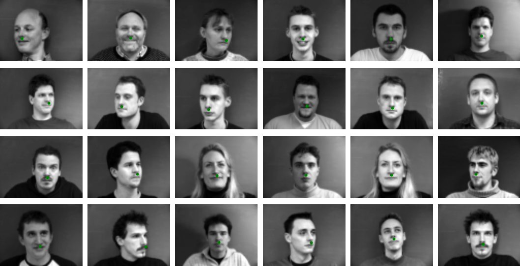
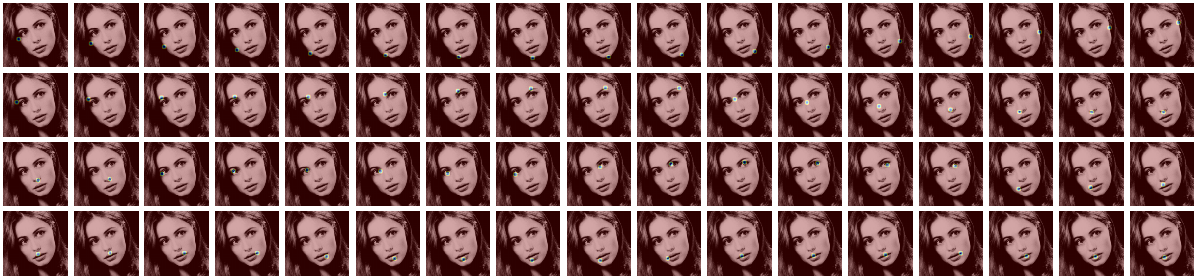
To start out, we'll use this labeled face database from the Informatics and Mathematical Modelling (IMM) group at the Technical University of Denmark. We'll randomize the order and divide into two groups: one size 192 for training and the other size 48 for testing. Below you can see a set of sample images from the training set along with their corresponding nose keypoint in green:
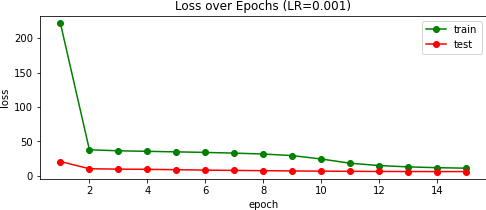
To the bottom-left, you can see the loss, measure by Mean Squared Error (MSE, L2 or Euclidean distance), of the model as it learns on the training set (green) and testing set (red).
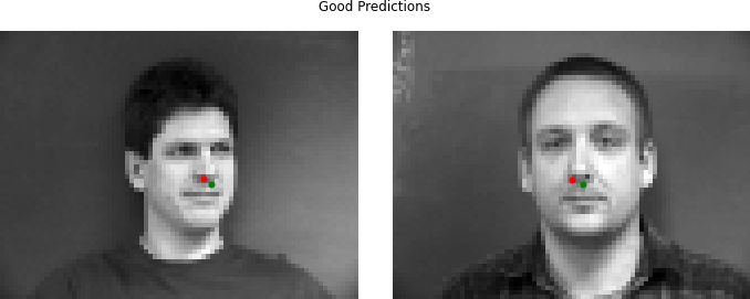
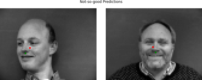
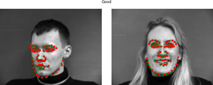
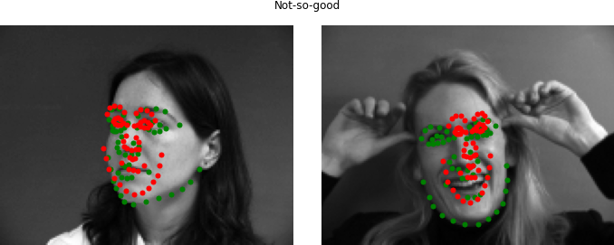
Below, you can see two good and bad predictions of the from the testing images. My hunch is that the model 'learns' the gradient from the shadow caused by the nose, but this itself is not a feature unique exclusively to the nose. As such, the network can be fooled by lips and facial hair, especially when an the head isn't oriented face-on or centered in the frame. These issues arise due to our small and similar dataset.
Full Facial Keypoints Detection
Dataset Augmentation
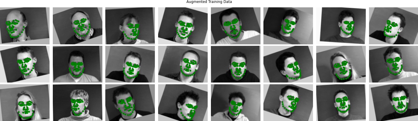
To cope with the model overfitting our dataset, and not learning the true features we want to for the sake of generalization, we can use data augmentation. This involves probabilistically altering our training set to artificially make it more diverse. I ended up $x$-shearing $\pm [0,8]\%$ and shifting up-down and left-right by $\pm [0,10]\%$, zooming out $[0, 20]\%$ to account for different scales, then rotating $\pm [0, 22]^{\circ}$.
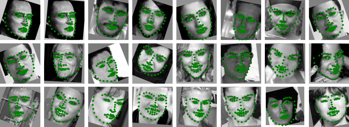
To accomplish all this, I used imgaug which is a very nice augmentation library. All of its functions can operate not only on images, but also operate on the keypoints as well. Below you can see the new, augmented training set :
Model
As for the actual network architecture, I drew inspiration from the Very Deep Convolutional Networks (VGG) paper. Notably, I used $3\times 3$ convolutions, and with a stride of 2 on channels of the same input-output size, $C$. Using stride 2 here captures the same receptive field of a $5\times 5$ convolution, but involves just $18C^2$ parameters and $18C^2HW$ FLOPS rather than $25C^2$ and $25C^2HW$. All of these convolutions were preceded by ReLU, and on the same-size layers I finished with a stride-2, $2\times2$ max pooling layer to ensure invariance to small spatial shifts before doubling the number of filter channels:
FaceNet(
(l1): Sequential(
(0): Conv2d(1, 16, kernel_size=(3, 3), stride=(2, 2))
(1): ReLU()
)
(l2): Sequential(
(0): Conv2d(16, 16, kernel_size=(3, 3), stride=(2, 2))
(1): ReLU()
(2): MaxPool2d(kernel_size=2, stride=2, padding=0, dilation=1, ceil_mode=False)
)
(l3): Sequential(
(0): Conv2d(16, 32, kernel_size=(3, 3), stride=(1, 1))
(1): ReLU()
)
(l4): Sequential(
(0): Conv2d(32, 32, kernel_size=(3, 3), stride=(1, 1))
(1): ReLU()
(2): MaxPool2d(kernel_size=2, stride=2, padding=0, dilation=1, ceil_mode=False)
)
(fc0): Sequential(
(0): Flatten(start_dim=1, end_dim=-1)
(1): Dropout(p=0.5, inplace=False)
(2): Linear(in_features=1120, out_features=512, bias=True)
(3): ReLU()
)
(fc1): Sequential(
(0): Linear(in_features=512, out_features=116, bias=True)
)
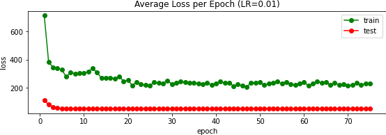
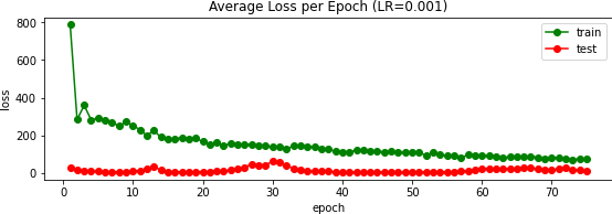
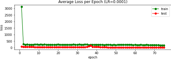
)I trained this network over 75 epochs using the AdamW optimizer (Adam with weight decay) along with the MSE error metric again. Experimentally, I found that a learning rate of $10^{-3}$ worked well versus $10^{-2}$ and $10^{-4}$:
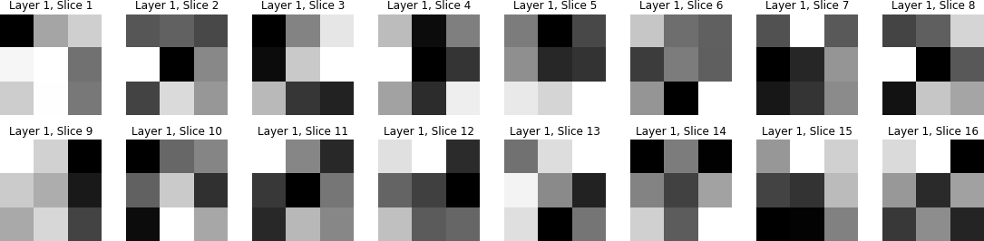
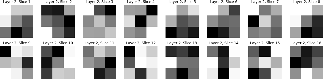
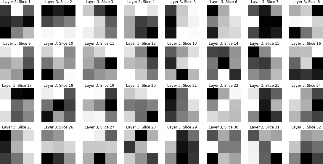
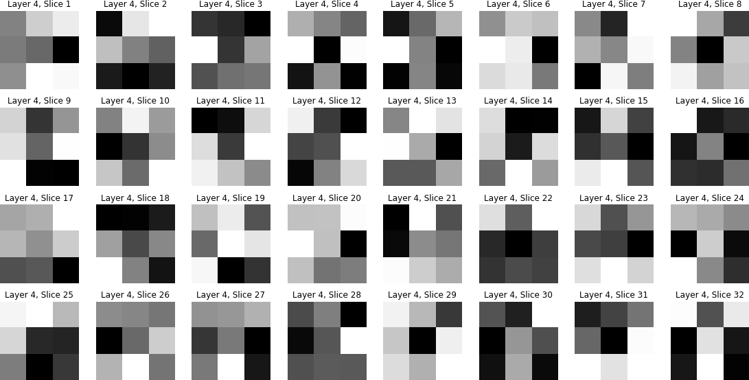
Below are the four learned convolutional filters. Most of them don't appear to be much of anything, but I suppose you could say some look similar to an edge detector (e.x. see project 2).
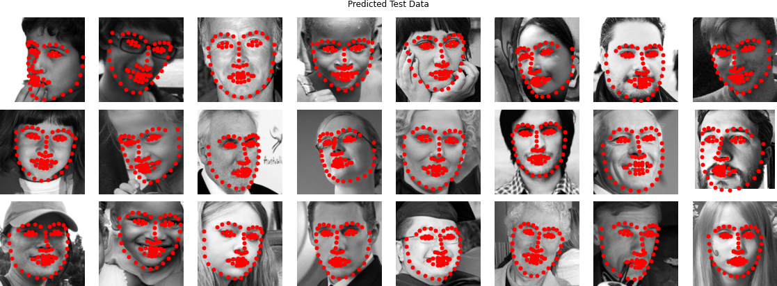
Two good and two bad examples of the network's predictions (red) are shown below. It certainly works better than the prior nose network, but still has some faults. You can see that the network sometimes struggles to properly project the points onto the face and doesn't perform well when it faces unusual poses.
Train With Larger Dataset
Next, we will use the Faces in the Wild dataset from the Intelligent Behavior Understanding Group (IBUG) at the Imperial College London. The dataset contains 6,666 labelled images of faces with 68 keypoints which we we split 80/20% into training/testing as before.
Augmentation
As for augmentation, we will perform the same process as before. Fortunately, the dataset also includes mirrored copies of the images with the correctly oriented left-right keypoints of each pair so we do not suffer from the mirroring issue.
One downside of this 'in-the-wild' dataset is that some faces are not fully included in the image, resulting in some of the keypoints being guessed + placed outside of the image. For these samples, I simply skipped adding them to the training data. Since these images are not initially squares, we need to crop to the given bounding box. However, this is fairly tight and I ended up enlarging it by 20% before cropping.
Additionally, sometimes the augmentation caused points to fall outside of the image due to the small margins from points to the edge. To resolve this, I attempted up to 5 different (random) augmentations before skipping to the subsequent sample. This is why there are occasional duplicate images. Because we have a huge dataset and because we are applying different augmentations each call, these duplicates do not meaningfully contribute to overfitting. Below you can see images from the training data:
Model
For the network, I modified ResNet-50 such that the input convolution layer took in a single (black and white) channel instead of the usual 3 (for color) with a kernel of size $7 \times 7$, stride-2, padding-3. I then changed the final linear layer to go from 2048 to 136 (68 points * 2 coordinates) and imported the pretrained weights from the original model. You can click the button below to see the behemoth model details:
Reveal Model Architecture
ResNet(
  (conv1): Conv2d(1, 64, kernel_size=(7, 7), stride=(2, 2), padding=(3, 3), bias=False)
  (bn1): BatchNorm2d(64, eps=1e-05, momentum=0.1, affine=True, track_running_stats=True)
  (relu): ReLU(inplace=True)
  (maxpool): MaxPool2d(kernel_size=3, stride=2, padding=1, dilation=1, ceil_mode=False)
  (layer1): Sequential(
    (0): Bottleneck(
      (conv1): Conv2d(64, 64, kernel_size=(1, 1), stride=(1, 1), bias=False)
      (bn1): BatchNorm2d(64, eps=1e-05, momentum=0.1, affine=True, track_running_stats=True)
      (conv2): Conv2d(64, 64, kernel_size=(3, 3), stride=(1, 1), padding=(1, 1), bias=False)
      (bn2): BatchNorm2d(64, eps=1e-05, momentum=0.1, affine=True, track_running_stats=True)
      (conv3): Conv2d(64, 256, kernel_size=(1, 1), stride=(1, 1), bias=False)
      (bn3): BatchNorm2d(256, eps=1e-05, momentum=0.1, affine=True, track_running_stats=True)
      (relu): ReLU(inplace=True)
      (downsample): Sequential(
        (0): Conv2d(64, 256, kernel_size=(1, 1), stride=(1, 1), bias=False)
        (1): BatchNorm2d(256, eps=1e-05, momentum=0.1, affine=True, track_running_stats=True)
      )
    )
    (1): Bottleneck(
      (conv1): Conv2d(256, 64, kernel_size=(1, 1), stride=(1, 1), bias=False)
      (bn1): BatchNorm2d(64, eps=1e-05, momentum=0.1, affine=True, track_running_stats=True)
      (conv2): Conv2d(64, 64, kernel_size=(3, 3), stride=(1, 1), padding=(1, 1), bias=False)
      (bn2): BatchNorm2d(64, eps=1e-05, momentum=0.1, affine=True, track_running_stats=True)
      (conv3): Conv2d(64, 256, kernel_size=(1, 1), stride=(1, 1), bias=False)
      (bn3): BatchNorm2d(256, eps=1e-05, momentum=0.1, affine=True, track_running_stats=True)
      (relu): ReLU(inplace=True)
    )
    (2): Bottleneck(
      (conv1): Conv2d(256, 64, kernel_size=(1, 1), stride=(1, 1), bias=False)
      (bn1): BatchNorm2d(64, eps=1e-05, momentum=0.1, affine=True, track_running_stats=True)
      (conv2): Conv2d(64, 64, kernel_size=(3, 3), stride=(1, 1), padding=(1, 1), bias=False)
      (bn2): BatchNorm2d(64, eps=1e-05, momentum=0.1, affine=True, track_running_stats=True)
      (conv3): Conv2d(64, 256, kernel_size=(1, 1), stride=(1, 1), bias=False)
      (bn3): BatchNorm2d(256, eps=1e-05, momentum=0.1, affine=True, track_running_stats=True)
      (relu): ReLU(inplace=True)
    )
  )
  (layer2): Sequential(
    (0): Bottleneck(
      (conv1): Conv2d(256, 128, kernel_size=(1, 1), stride=(1, 1), bias=False)
      (bn1): BatchNorm2d(128, eps=1e-05, momentum=0.1, affine=True, track_running_stats=True)
      (conv2): Conv2d(128, 128, kernel_size=(3, 3), stride=(2, 2), padding=(1, 1), bias=False)
      (bn2): BatchNorm2d(128, eps=1e-05, momentum=0.1, affine=True, track_running_stats=True)
      (conv3): Conv2d(128, 512, kernel_size=(1, 1), stride=(1, 1), bias=False)
      (bn3): BatchNorm2d(512, eps=1e-05, momentum=0.1, affine=True, track_running_stats=True)
      (relu): ReLU(inplace=True)
      (downsample): Sequential(
        (0): Conv2d(256, 512, kernel_size=(1, 1), stride=(2, 2), bias=False)
        (1): BatchNorm2d(512, eps=1e-05, momentum=0.1, affine=True, track_running_stats=True)
      )
    )
    (1): Bottleneck(
      (conv1): Conv2d(512, 128, kernel_size=(1, 1), stride=(1, 1), bias=False)
      (bn1): BatchNorm2d(128, eps=1e-05, momentum=0.1, affine=True, track_running_stats=True)
      (conv2): Conv2d(128, 128, kernel_size=(3, 3), stride=(1, 1), padding=(1, 1), bias=False)
      (bn2): BatchNorm2d(128, eps=1e-05, momentum=0.1, affine=True, track_running_stats=True)
      (conv3): Conv2d(128, 512, kernel_size=(1, 1), stride=(1, 1), bias=False)
      (bn3): BatchNorm2d(512, eps=1e-05, momentum=0.1, affine=True, track_running_stats=True)
      (relu): ReLU(inplace=True)
    )
    (2): Bottleneck(
      (conv1): Conv2d(512, 128, kernel_size=(1, 1), stride=(1, 1), bias=False)
      (bn1): BatchNorm2d(128, eps=1e-05, momentum=0.1, affine=True, track_running_stats=True)
      (conv2): Conv2d(128, 128, kernel_size=(3, 3), stride=(1, 1), padding=(1, 1), bias=False)
      (bn2): BatchNorm2d(128, eps=1e-05, momentum=0.1, affine=True, track_running_stats=True)
      (conv3): Conv2d(128, 512, kernel_size=(1, 1), stride=(1, 1), bias=False)
      (bn3): BatchNorm2d(512, eps=1e-05, momentum=0.1, affine=True, track_running_stats=True)
      (relu): ReLU(inplace=True)
    )
    (3): Bottleneck(
      (conv1): Conv2d(512, 128, kernel_size=(1, 1), stride=(1, 1), bias=False)
      (bn1): BatchNorm2d(128, eps=1e-05, momentum=0.1, affine=True, track_running_stats=True)
      (conv2): Conv2d(128, 128, kernel_size=(3, 3), stride=(1, 1), padding=(1, 1), bias=False)
      (bn2): BatchNorm2d(128, eps=1e-05, momentum=0.1, affine=True, track_running_stats=True)
      (conv3): Conv2d(128, 512, kernel_size=(1, 1), stride=(1, 1), bias=False)
      (bn3): BatchNorm2d(512, eps=1e-05, momentum=0.1, affine=True, track_running_stats=True)
      (relu): ReLU(inplace=True)
    )
  )
  (layer3): Sequential(
    (0): Bottleneck(
      (conv1): Conv2d(512, 256, kernel_size=(1, 1), stride=(1, 1), bias=False)
      (bn1): BatchNorm2d(256, eps=1e-05, momentum=0.1, affine=True, track_running_stats=True)
      (conv2): Conv2d(256, 256, kernel_size=(3, 3), stride=(2, 2), padding=(1, 1), bias=False)
      (bn2): BatchNorm2d(256, eps=1e-05, momentum=0.1, affine=True, track_running_stats=True)
      (conv3): Conv2d(256, 1024, kernel_size=(1, 1), stride=(1, 1), bias=False)
      (bn3): BatchNorm2d(1024, eps=1e-05, momentum=0.1, affine=True, track_running_stats=True)
      (relu): ReLU(inplace=True)
      (downsample): Sequential(
        (0): Conv2d(512, 1024, kernel_size=(1, 1), stride=(2, 2), bias=False)
        (1): BatchNorm2d(1024, eps=1e-05, momentum=0.1, affine=True, track_running_stats=True)
      )
    )
    (1): Bottleneck(
      (conv1): Conv2d(1024, 256, kernel_size=(1, 1), stride=(1, 1), bias=False)
      (bn1): BatchNorm2d(256, eps=1e-05, momentum=0.1, affine=True, track_running_stats=True)
      (conv2): Conv2d(256, 256, kernel_size=(3, 3), stride=(1, 1), padding=(1, 1), bias=False)
      (bn2): BatchNorm2d(256, eps=1e-05, momentum=0.1, affine=True, track_running_stats=True)
      (conv3): Conv2d(256, 1024, kernel_size=(1, 1), stride=(1, 1), bias=False)
      (bn3): BatchNorm2d(1024, eps=1e-05, momentum=0.1, affine=True, track_running_stats=True)
      (relu): ReLU(inplace=True)
    )
    (2): Bottleneck(
      (conv1): Conv2d(1024, 256, kernel_size=(1, 1), stride=(1, 1), bias=False)
      (bn1): BatchNorm2d(256, eps=1e-05, momentum=0.1, affine=True, track_running_stats=True)
      (conv2): Conv2d(256, 256, kernel_size=(3, 3), stride=(1, 1), padding=(1, 1), bias=False)
      (bn2): BatchNorm2d(256, eps=1e-05, momentum=0.1, affine=True, track_running_stats=True)
      (conv3): Conv2d(256, 1024, kernel_size=(1, 1), stride=(1, 1), bias=False)
      (bn3): BatchNorm2d(1024, eps=1e-05, momentum=0.1, affine=True, track_running_stats=True)
      (relu): ReLU(inplace=True)
    )
    (3): Bottleneck(
      (conv1): Conv2d(1024, 256, kernel_size=(1, 1), stride=(1, 1), bias=False)
      (bn1): BatchNorm2d(256, eps=1e-05, momentum=0.1, affine=True, track_running_stats=True)
      (conv2): Conv2d(256, 256, kernel_size=(3, 3), stride=(1, 1), padding=(1, 1), bias=False)
      (bn2): BatchNorm2d(256, eps=1e-05, momentum=0.1, affine=True, track_running_stats=True)
      (conv3): Conv2d(256, 1024, kernel_size=(1, 1), stride=(1, 1), bias=False)
      (bn3): BatchNorm2d(1024, eps=1e-05, momentum=0.1, affine=True, track_running_stats=True)
      (relu): ReLU(inplace=True)
    )
    (4): Bottleneck(
      (conv1): Conv2d(1024, 256, kernel_size=(1, 1), stride=(1, 1), bias=False)
      (bn1): BatchNorm2d(256, eps=1e-05, momentum=0.1, affine=True, track_running_stats=True)
      (conv2): Conv2d(256, 256, kernel_size=(3, 3), stride=(1, 1), padding=(1, 1), bias=False)
      (bn2): BatchNorm2d(256, eps=1e-05, momentum=0.1, affine=True, track_running_stats=True)
      (conv3): Conv2d(256, 1024, kernel_size=(1, 1), stride=(1, 1), bias=False)
      (bn3): BatchNorm2d(1024, eps=1e-05, momentum=0.1, affine=True, track_running_stats=True)
      (relu): ReLU(inplace=True)
    )
    (5): Bottleneck(
      (conv1): Conv2d(1024, 256, kernel_size=(1, 1), stride=(1, 1), bias=False)
      (bn1): BatchNorm2d(256, eps=1e-05, momentum=0.1, affine=True, track_running_stats=True)
      (conv2): Conv2d(256, 256, kernel_size=(3, 3), stride=(1, 1), padding=(1, 1), bias=False)
      (bn2): BatchNorm2d(256, eps=1e-05, momentum=0.1, affine=True, track_running_stats=True)
      (conv3): Conv2d(256, 1024, kernel_size=(1, 1), stride=(1, 1), bias=False)
      (bn3): BatchNorm2d(1024, eps=1e-05, momentum=0.1, affine=True, track_running_stats=True)
      (relu): ReLU(inplace=True)
    )
  )
  (layer4): Sequential(
    (0): Bottleneck(
      (conv1): Conv2d(1024, 512, kernel_size=(1, 1), stride=(1, 1), bias=False)
      (bn1): BatchNorm2d(512, eps=1e-05, momentum=0.1, affine=True, track_running_stats=True)
      (conv2): Conv2d(512, 512, kernel_size=(3, 3), stride=(2, 2), padding=(1, 1), bias=False)
      (bn2): BatchNorm2d(512, eps=1e-05, momentum=0.1, affine=True, track_running_stats=True)
      (conv3): Conv2d(512, 2048, kernel_size=(1, 1), stride=(1, 1), bias=False)
      (bn3): BatchNorm2d(2048, eps=1e-05, momentum=0.1, affine=True, track_running_stats=True)
      (relu): ReLU(inplace=True)
      (downsample): Sequential(
        (0): Conv2d(1024, 2048, kernel_size=(1, 1), stride=(2, 2), bias=False)
        (1): BatchNorm2d(2048, eps=1e-05, momentum=0.1, affine=True, track_running_stats=True)
      )
    )
    (1): Bottleneck(
      (conv1): Conv2d(2048, 512, kernel_size=(1, 1), stride=(1, 1), bias=False)
      (bn1): BatchNorm2d(512, eps=1e-05, momentum=0.1, affine=True, track_running_stats=True)
      (conv2): Conv2d(512, 512, kernel_size=(3, 3), stride=(1, 1), padding=(1, 1), bias=False)
      (bn2): BatchNorm2d(512, eps=1e-05, momentum=0.1, affine=True, track_running_stats=True)
      (conv3): Conv2d(512, 2048, kernel_size=(1, 1), stride=(1, 1), bias=False)
      (bn3): BatchNorm2d(2048, eps=1e-05, momentum=0.1, affine=True, track_running_stats=True)
      (relu): ReLU(inplace=True)
    )
    (2): Bottleneck(
      (conv1): Conv2d(2048, 512, kernel_size=(1, 1), stride=(1, 1), bias=False)
      (bn1): BatchNorm2d(512, eps=1e-05, momentum=0.1, affine=True, track_running_stats=True)
      (conv2): Conv2d(512, 512, kernel_size=(3, 3), stride=(1, 1), padding=(1, 1), bias=False)
      (bn2): BatchNorm2d(512, eps=1e-05, momentum=0.1, affine=True, track_running_stats=True)
      (conv3): Conv2d(512, 2048, kernel_size=(1, 1), stride=(1, 1), bias=False)
      (bn3): BatchNorm2d(2048, eps=1e-05, momentum=0.1, affine=True, track_running_stats=True)
      (relu): ReLU(inplace=True)
    )
  )
  (avgpool): AdaptiveAvgPool2d(output_size=(1, 1))
  (fc): Linear(in_features=2048, out_features=136, bias=True)
)
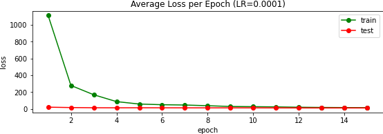
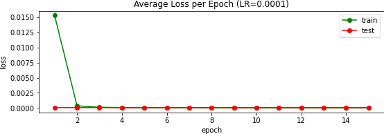
In our class's Kaggle competition, this scored an error of 13.32866; my user name is Max Vogel. Above you can see a few of the predictions, and to the right the validation loss over 15 epochs.
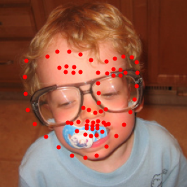
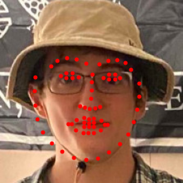
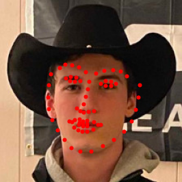
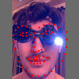
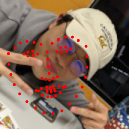
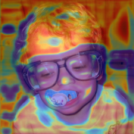
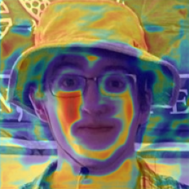
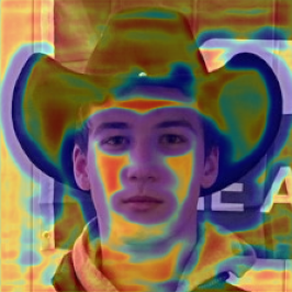
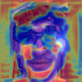
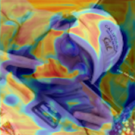
Below are a couple of my own personal photos. The model gets a little confused with hats, but worked surprisingly not-terribly on the image of Jack with the jewelers glasses + lense flair. Unfortunately baby-me was all over the place and Frank winning at poker didn't work out so well either.
Pixelwise Classification
Rather than predicting the location of the keypoints, we can look at this as a classification problem: for every pixel, how likely is it that it is part of a keypoint?
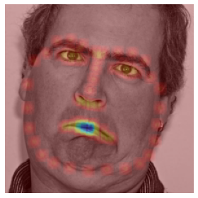
This will involve altering our dataset such that rather than 68 single points we will have 68 heat maps. To go about generating these heat maps, I created a heatmap for each of the keypoints by placing a 2D Gaussian with a kernel size $16$ and $\sigma = 5$. As shown to the right, we can sum all of these heatmaps together to get a single heatmap for the entire image. Due to the fact that it is expensive to generate these heatmaps, I did not implement any other data augmentation besides cropping to the bounding box and resizing to $224 \times 224$.
Model
As for the model, I modified the U-Net architecture
such
that it took in a single channel and output 68. Below you can click to reveal the full model
summary:
Reveal Model Architecture
UNet(
  (encoder1): Sequential(
    (enc1conv1): Conv2d(1, 32, kernel_size=(3, 3), stride=(1, 1), padding=(1, 1), bias=False)
    (enc1norm1): BatchNorm2d(32, eps=1e-05, momentum=0.1, affine=True, track_running_stats=True)
    (enc1relu1): ReLU(inplace=True)
    (enc1conv2): Conv2d(32, 32, kernel_size=(3, 3), stride=(1, 1), padding=(1, 1), bias=False)
    (enc1norm2): BatchNorm2d(32, eps=1e-05, momentum=0.1, affine=True, track_running_stats=True)
    (enc1relu2): ReLU(inplace=True)
  )
  (pool1): MaxPool2d(kernel_size=2, stride=2, padding=0, dilation=1, ceil_mode=False)
  (encoder2): Sequential(
    (enc2conv1): Conv2d(32, 64, kernel_size=(3, 3), stride=(1, 1), padding=(1, 1), bias=False)
    (enc2norm1): BatchNorm2d(64, eps=1e-05, momentum=0.1, affine=True, track_running_stats=True)
    (enc2relu1): ReLU(inplace=True)
    (enc2conv2): Conv2d(64, 64, kernel_size=(3, 3), stride=(1, 1), padding=(1, 1), bias=False)
    (enc2norm2): BatchNorm2d(64, eps=1e-05, momentum=0.1, affine=True, track_running_stats=True)
    (enc2relu2): ReLU(inplace=True)
  )
  (pool2): MaxPool2d(kernel_size=2, stride=2, padding=0, dilation=1, ceil_mode=False)
  (encoder3): Sequential(
    (enc3conv1): Conv2d(64, 128, kernel_size=(3, 3), stride=(1, 1), padding=(1, 1), bias=False)
    (enc3norm1): BatchNorm2d(128, eps=1e-05, momentum=0.1, affine=True, track_running_stats=True)
    (enc3relu1): ReLU(inplace=True)
    (enc3conv2): Conv2d(128, 128, kernel_size=(3, 3), stride=(1, 1), padding=(1, 1), bias=False)
    (enc3norm2): BatchNorm2d(128, eps=1e-05, momentum=0.1, affine=True, track_running_stats=True)
    (enc3relu2): ReLU(inplace=True)
  )
  (pool3): MaxPool2d(kernel_size=2, stride=2, padding=0, dilation=1, ceil_mode=False)
  (encoder4): Sequential(
    (enc4conv1): Conv2d(128, 256, kernel_size=(3, 3), stride=(1, 1), padding=(1, 1), bias=False)
    (enc4norm1): BatchNorm2d(256, eps=1e-05, momentum=0.1, affine=True, track_running_stats=True)
    (enc4relu1): ReLU(inplace=True)
    (enc4conv2): Conv2d(256, 256, kernel_size=(3, 3), stride=(1, 1), padding=(1, 1), bias=False)
    (enc4norm2): BatchNorm2d(256, eps=1e-05, momentum=0.1, affine=True, track_running_stats=True)
    (enc4relu2): ReLU(inplace=True)
  )
  (pool4): MaxPool2d(kernel_size=2, stride=2, padding=0, dilation=1, ceil_mode=False)
  (bottleneck): Sequential(
    (bottleneckconv1): Conv2d(256, 512, kernel_size=(3, 3), stride=(1, 1), padding=(1, 1), bias=False)
    (bottlenecknorm1): BatchNorm2d(512, eps=1e-05, momentum=0.1, affine=True, track_running_stats=True)
    (bottleneckrelu1): ReLU(inplace=True)
    (bottleneckconv2): Conv2d(512, 512, kernel_size=(3, 3), stride=(1, 1), padding=(1, 1), bias=False)
    (bottlenecknorm2): BatchNorm2d(512, eps=1e-05, momentum=0.1, affine=True, track_running_stats=True)
    (bottleneckrelu2): ReLU(inplace=True)
  )
  (upconv4): ConvTranspose2d(512, 256, kernel_size=(2, 2), stride=(2, 2))
  (decoder4): Sequential(
    (dec4conv1): Conv2d(512, 256, kernel_size=(3, 3), stride=(1, 1), padding=(1, 1), bias=False)
    (dec4norm1): BatchNorm2d(256, eps=1e-05, momentum=0.1, affine=True, track_running_stats=True)
    (dec4relu1): ReLU(inplace=True)
    (dec4conv2): Conv2d(256, 256, kernel_size=(3, 3), stride=(1, 1), padding=(1, 1), bias=False)
    (dec4norm2): BatchNorm2d(256, eps=1e-05, momentum=0.1, affine=True, track_running_stats=True)
    (dec4relu2): ReLU(inplace=True)
  )
  (upconv3): ConvTranspose2d(256, 128, kernel_size=(2, 2), stride=(2, 2))
  (decoder3): Sequential(
    (dec3conv1): Conv2d(256, 128, kernel_size=(3, 3), stride=(1, 1), padding=(1, 1), bias=False)
    (dec3norm1): BatchNorm2d(128, eps=1e-05, momentum=0.1, affine=True, track_running_stats=True)
    (dec3relu1): ReLU(inplace=True)
    (dec3conv2): Conv2d(128, 128, kernel_size=(3, 3), stride=(1, 1), padding=(1, 1), bias=False)
    (dec3norm2): BatchNorm2d(128, eps=1e-05, momentum=0.1, affine=True, track_running_stats=True)
    (dec3relu2): ReLU(inplace=True)
  )
  (upconv2): ConvTranspose2d(128, 64, kernel_size=(2, 2), stride=(2, 2))
  (decoder2): Sequential(
    (dec2conv1): Conv2d(128, 64, kernel_size=(3, 3), stride=(1, 1), padding=(1, 1), bias=False)
    (dec2norm1): BatchNorm2d(64, eps=1e-05, momentum=0.1, affine=True, track_running_stats=True)
    (dec2relu1): ReLU(inplace=True)
    (dec2conv2): Conv2d(64, 64, kernel_size=(3, 3), stride=(1, 1), padding=(1, 1), bias=False)
    (dec2norm2): BatchNorm2d(64, eps=1e-05, momentum=0.1, affine=True, track_running_stats=True)
    (dec2relu2): ReLU(inplace=True)
  )
  (upconv1): ConvTranspose2d(64, 32, kernel_size=(2, 2), stride=(2, 2))
  (decoder1): Sequential(
    (dec1conv1): Conv2d(64, 32, kernel_size=(3, 3), stride=(1, 1), padding=(1, 1), bias=False)
    (dec1norm1): BatchNorm2d(32, eps=1e-05, momentum=0.1, affine=True, track_running_stats=True)
    (dec1relu1): ReLU(inplace=True)
    (dec1conv2): Conv2d(32, 32, kernel_size=(3, 3), stride=(1, 1), padding=(1, 1), bias=False)
    (dec1norm2): BatchNorm2d(32, eps=1e-05, momentum=0.1, affine=True, track_running_stats=True)
    (dec1relu2): ReLU(inplace=True)
  )
  (conv): Conv2d(32, 68, kernel_size=(1, 1), stride=(1, 1))
)
To train this I used the same learning rate of $10^{-3}$ and AdamW optimizer from before, but now alongside the Cross Entropy loss function since we're now solving training a network that outputs a probabilistic guess. Additionally, I increased the batch size to 4, whereas in all prior stages it was simply 1. This has the effect of reducing the computation involved when training the network since the weights are updated after four images are processed (opposed to after every image).
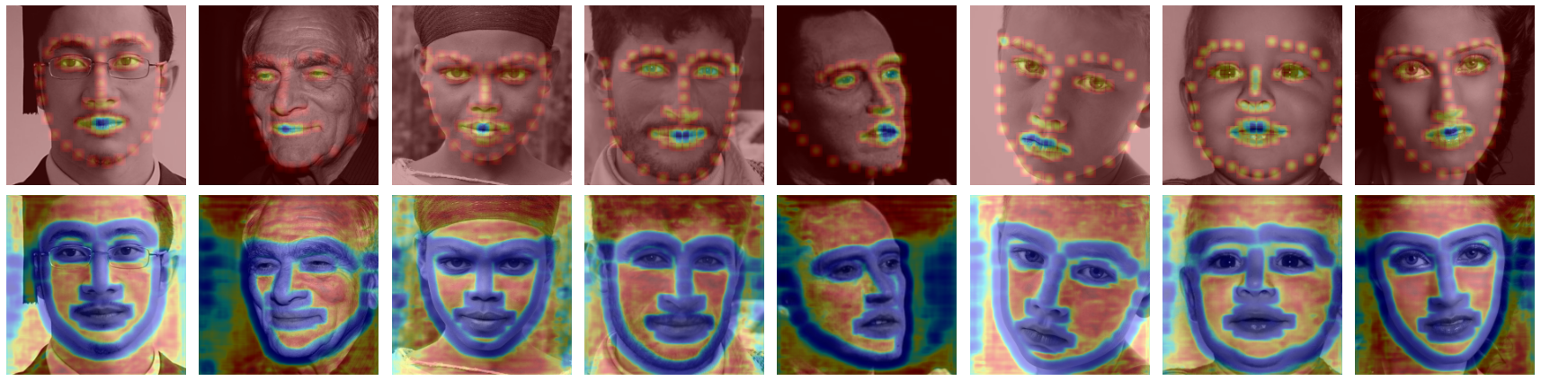
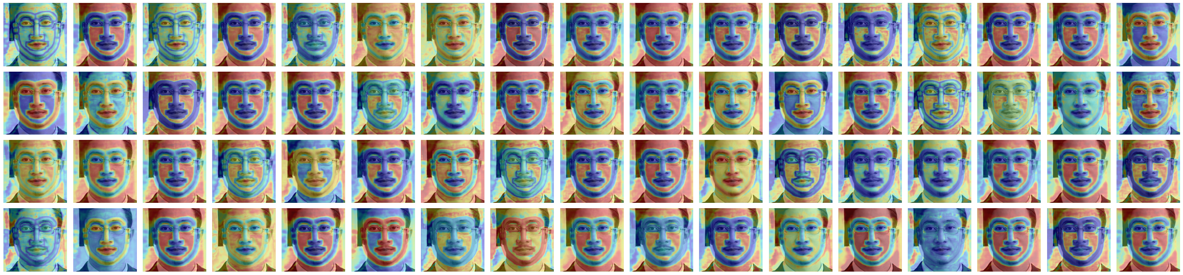
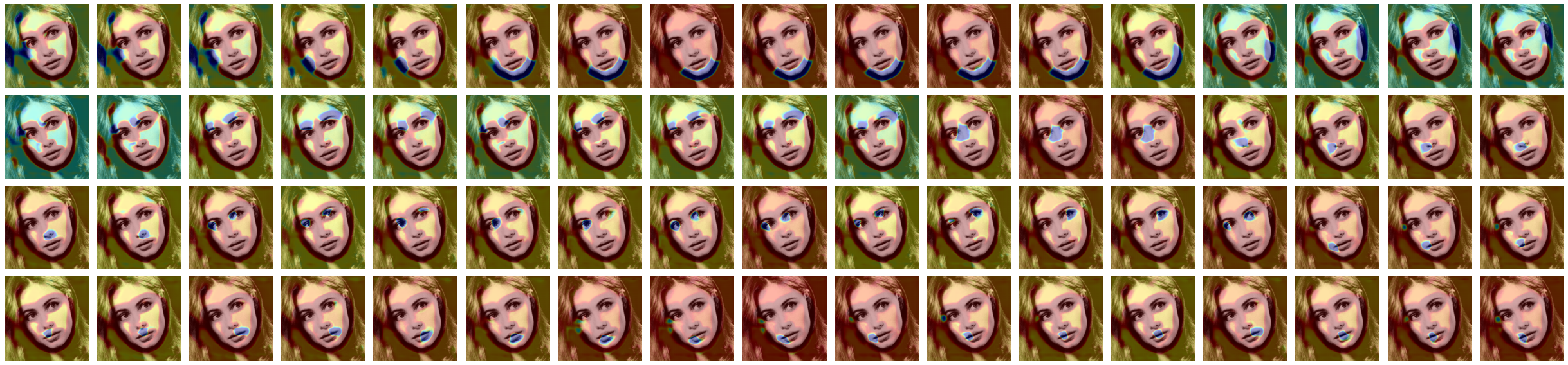
Because both storing or computing $224\times 224 \times 68 \approx 3 \cdot 10^6 $ pixels for each heatmap is painful, I naively summed the 68 output layers from the network and compared it to the summed ground truth heatmaps which were memoized. This allowed me to train the network in a reasonable amount of time, but had the downside of the network not having the fidelity to associate individual heatmaps with individual keypoints. This is why, as you can see below, the network is not able to predict the location of the keypoints as well as the previous model. In the first image below, the top row are the 'true' heatmaps while the bottom are what the model spits out. In the subsequent image you can also see all of the similar 68 output layers for the first testing image.
To (attempt to) work around this, I bit the bullet and ended up forking over $20 to Google so that I could use their phat computers that are capable of storing these 68 heatmaps for each image. Even with this, I ended up limiting the dataset to 3,000 images as I was still running low on memory.
Now, when training, the 68 output channels from the model could be compared with all 68 (memoized) ground-truth heatmaps by measure of the Mean Absolute Error (MAE, L1 norm). In theory, this should encourage the network to become more sparse. In practice, I wasn't able to manage to dial in the hyperparameters to get the network to converge before running out of credits, time, and sanity. Unfortunate!
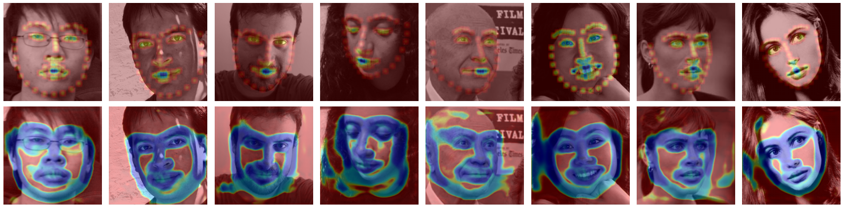
Below you can see the prediction results in the same format as above. Additionally, you can hover over the 68 channels picture to see how each of the predictions compare versus their respective ground-truth heatmaps. Some kind of have the right idea, and this gives me hope that had I been able to train over more epochs and had more time to tune the hyperparameters that this could work.
All in all, despite all the hiccups along the way, I thoroughly enjoyed this project. I used an amalgamation of skills I've picked up over the course of this course and I can confidently say that I am much more proficient in navigating/understanding documentation as well as implementing code from scratch.